library(xts)
library(jsonlite)

tix <- c('FMAGX', 'IWD', 'IWF', 'IWN', 'IWO', 'IVV')

download_tiingo <- function(ticker, t_api) {

  t_url <- paste0('https://api.tiingo.com/tiingo/daily/',
                  ticker,
                  '/prices?startDate=1970-01-01',
                  '&endDate=2024-03-26',
                  '&token=', t_api)
  dat <- jsonlite::read_json(t_url)
  date_raw <- sapply(dat, '[[', 'date')
  date_vec <- as.Date(date_raw)
  price_vec <- sapply(dat, '[[', 'adjClose')
  price <- xts(price_vec, date_vec)
  colnames(price) <- ticker
  ret <- price / lag.xts(price, 1) - 1
  return(ret[-1, ])
}

d_list <- lapply(tix, download_tiingo, t_api)
ret_union <- do.call('cbind', d_list)
ret <- na.omit(ret_union)Intro
Style analysis is a great tool to see how consistent managers have been in their investment approach.
For equity managers this is commonly measured by the Morningstar Style Box. We can readily see on Morningstar dot com how mutual funds and ETFs are positioned in this box based on their latest holdings. However, a history of how their style has drifted (or remained constant) over the years isn’t commonly published.
This post will demonstrate an open source solution that can solve for both current style and how it has tracked over time. We are going to use a returns-based solution that has the advantage of needing less observations, i.e., we only need the historical returns as opposed to a history of all the fund and style indices (or factors) holdings. The returns based approach dates back to William Sharpe’s work in the late 1980s and early 1990s, for example, see ASSET ALLOCATION: MANAGEMENT STYLE AND PERFORMANCE MEASUREMENT. The returns-based framework is deployed in a variety of commercial software including MPI Stylus, Zephyr, and Factset’s SPAR.
Gathering Data for the Experiment
As an example this post will use a well known growth fund with a long track record, the Fidelity Magellan Fund (FMAGX), and iShares index ETFs to represent the value and growth indices of the Russell 1000 and 2000.
The code snippet below downloads the returns from tiingo. If you want to follow along / reproduce this example you can follow the link to register for a free api key. I’ve hidden mine, so you will need to set the variable t_api below to your api key. The ending result ret is the time-series of returns we need for our example.
The Algorithm
The heart of the style analysis is a tracking error minimization problem. We solve for a “portfolio” that allocates to our style indices (e.g., Russell 1000 Growth, Russell 1000 Value, Russell 2000 Growth, Russell 2000 Value) in a way that minimizes its tracking error to the manager.
The TE minimization goal is a quadratic optimization. In the linked article above Sharpe discusses Markowitz’s Critical Line Algorithm and a gradient descent method as options to solve for the weights. However, I’m going to leave the Critical Line Algorithm for another post and showcase a general purpose quadratic solver: the R quadprog package.
As described in the package manual, the quadprog routine uses the dual method of Goldfarb and Idnani (1982, 1983) via the form \(min(-d^Tb + 1/2b^TDb)\) with the constraints \(A^Tb >= b_0\).
\(b\) and \(d\) are an \(n\) vectors, in this case \(d\) is the vector containing the \(n\) covariances of each factor indices with the manager. \(b\) is the vector we are trying to solve for that contains the weight of each style index.
\(D\) is the an \(n * n\) matrix, in this case it’s the covariance matrix of the \(n\) style indices.
\(A\) and \(b_0\) are the constraints, \(A\) is a matrix and \(b_0\) is a vector:
It’s easier (for me at least) to think of A transposed, \(A^T\), when going through the three constraints below:
Weights sum to 1 (100%) constraint: The first row of \(A^T\) is \(n\) 1s to correspond with the first row of \(b_0\) (a column vector) also being a 1.
Upperbound weight constraint of 100%: Below the one row is an \(n * n\) diagonal matrix of -1s. This will correspond with \(n\) -1s in the rows of \(b_0\).
Lowerbound weight constraint of 0%: Below the upperbound matrix is another \(n * n\)diagonal matrix of 1s (an identity matrix). This will correspond with \(n\) 0s in the \(b_0\) vector.
In our case \(n = 4\), leading to:
\[A^T = \begin{bmatrix} 1 & 1 & 1 & 1 \\ -1 & 0 & 0 & 0 \\ 0 & -1 & 0 & 0 \\ 0 & 0 & -1 & 0 \\ 0 & 0 & 0 & -1 \\ 1 & 0 & 0 & 0 \\ 0 & 1 & 0 & 0 \\ 0 & 0 & 1 & 0 \\ 0 & 0 & 0 & 1 \end{bmatrix} b_0 = \begin{bmatrix} 1 \\ -1 \\ - 1 \\ -1 \\ -1 \\ 1 \\ 1 \\ 1 \\ 1 \end{bmatrix}\]
Implementation
We’ll need an R function that takes the fund and style indices as inputs, set’s up \(d, D, A, b_0\) and uses quadprog to solve for \(b\).
solve_style_wgt <- function(fund, fact) {
  # fund = manager returns
  # fact = factor or style indices
  n_fact <- ncol(fact) # n
  cov_fact <- cov(fact) # D
  cov_vec <- matrix(nrow = n_fact, ncol = 1) # d
  for (i in 1:n_fact) {
    cov_vec[i, 1] <- cov(fact[, i], fund)
  }
  a_mat_t <- rbind(rep(1, n_fact), diag(-1, n_fact), diag(1, n_fact)) # A'
  a_mat <- t(a_mat_t)
  b_0 <- c(1, rep(-1, n_fact), rep(0, n_fact))
  res <- quadprog::solve.QP(cov_fact, cov_vec, a_mat, bvec = b_0, meq = 1)
  return(res)
}
A note on the meq argument in the solve.QP function. The constraints in quadratic optimization can either be equality = conditions or inequality >= conditions. In our case the first constraint is an equality: sum of \(b = 1\). The lower and upper bounds are inequalities: e.g., the lower bound for each \(b >= 0\). Setting meq to 1 tells the optimizer the first constraint is an equality and the remaining constraints are inequalities.
Here’s a recent test of the function to see how the fund’s been positioned since 2019.
style_ind <- ret['2019/', 2:5]
fund <- ret['2019/', 1]
res <- solve_style_wgt(fund, style_ind)
res
$solution
[1] 1.288061e-01 8.711939e-01 9.929143e-18 0.000000e+00
$value
[1] -0.0001008058
$unconstrained.solution
[1] 0.31028681 0.79937551 -0.18470617 0.08095713
$iterations
[1] 4 0
$Lagrangian
[1] 3.592584e-06 0.000000e+00 0.000000e+00 0.000000e+00 0.000000e+00
[6] 0.000000e+00 0.000000e+00 6.343881e-06 3.305878e-06
$iact
[1] 8 9 1The $solution is the weights we are after. A quick way to visualize the style weights is with a barplot. We can also create a portfolio that invests in the style weights to check the fit by measuring the r-squared between the style weights and the manager.
barplot(res$solution, names.arg=  c("Large Value", "Large Growth", "Small Value",
                                    "Small Growth"))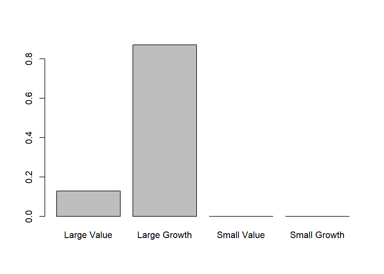
style_port <- rowSums(matrix(res$solution, nrow = nrow(ret['2019/']), ncol = 4,
                             byrow = TRUE) * style_ind)
r2 <- cor(fund, style_port)^2
cum_ret <- apply(cbind(style_port, fund) + 1, 2, cumprod)
wealth <- xts(cum_ret, zoo::index(fund))
plot(wealth, legend.loc = 'topleft')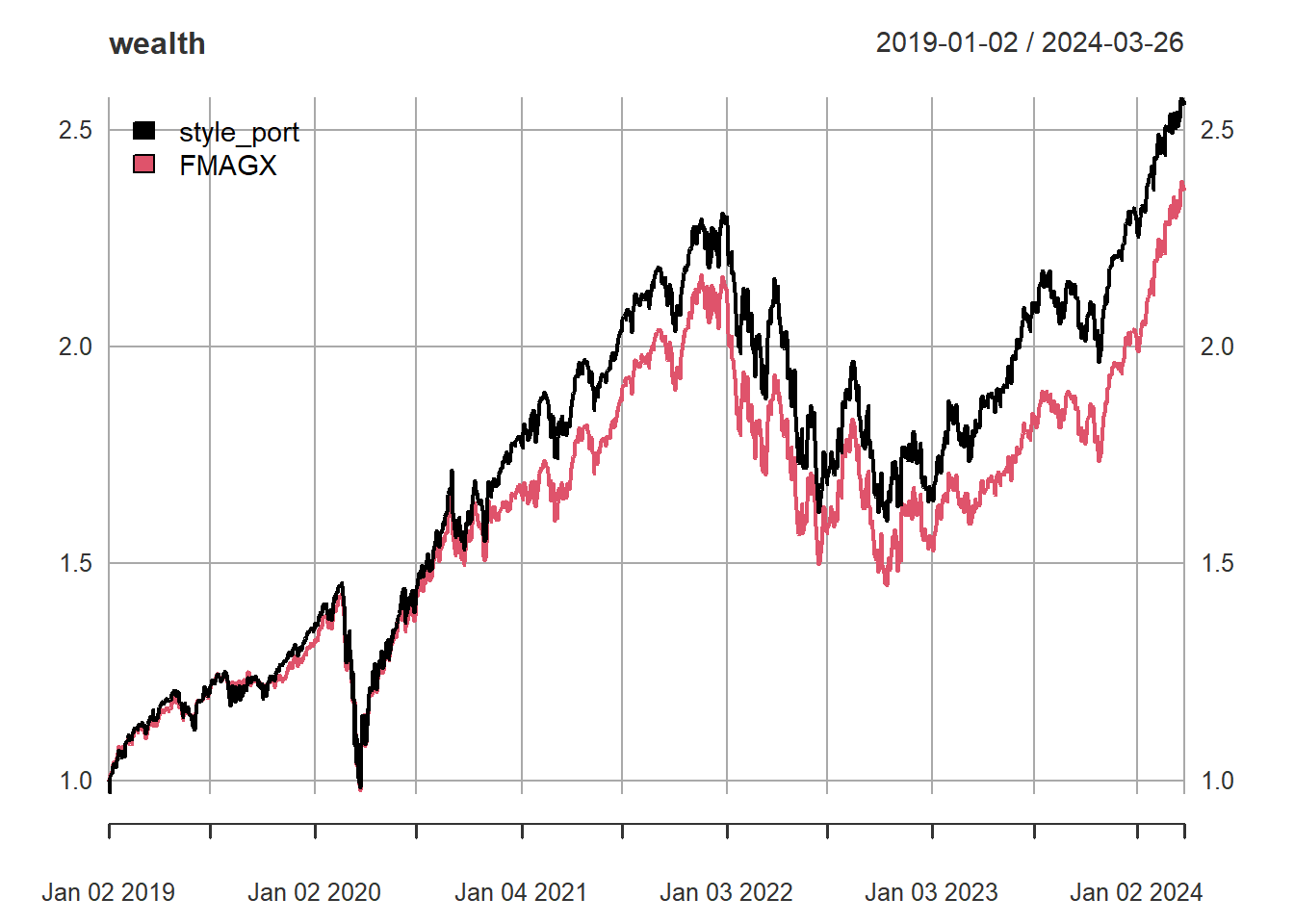
paste0('r-squared = ', round(r2 * 100, 1), '%')[1] "r-squared = 96.6%"We can also use an x-y plot to mimic the Morningstar Style Box. One way to do this is to set the four style indexes at x, y points (one could expand to 9 to include mid-cap to if desired):
Large Value = (-1, 1)
Large Growth = (1, 1)
Small Value = (-1, -1)
Small Growth = (-1, 1)
Then we map the fund’s style weights by:
x = large growth + small growth - large value - small value
y = large growth + large value - small growth - small value
As you can see a fund with small growth and large value weights would have a negative x coordinate near the left side of the box and similarly a fund with more large cap weights would have a positive y coordinate near the top of the box.
library(ggplot2)
library(ggrepel)
plot_style <- function(res) {
  x <- res$solution[2] + res$solution[4] - res$solution[1] - res$solution[3]
  y <- res$solution[1] + res$solution[2] - res$solution[3] - res$solution[4]
  df <- data.frame(
    x = c(x, -1, 1, -1, 1),
    y = c(y, 1, 1, -1, -1),
    name = c('Manager', 'Large Value', 'Large Growth', 'Small Value', 'Small Growth'),
    type = c('Manager', rep('Reference', 4))
  )
  ggplot(df, aes(x = x, y = y, label = name, color = type)) +
    geom_point() +
    scale_x_continuous(limits = c(-1.2, 1.2), breaks = c(-1, 0, 1)) +
    scale_y_continuous(limits = c(-1.2, 1.2), breaks = c(-1, 0, 1)) +
    geom_label_repel() +
    ylab('') + xlab('') +
    theme_linedraw() +
    theme(legend.position = 'none')
}
plot_style(res)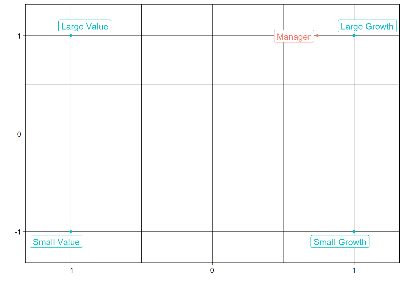
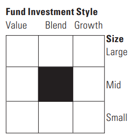
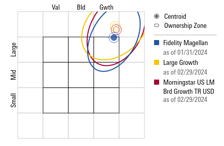
The plot highlights the large cap growth tilt of the manager using returns since 2019. This matches the style box pulled from it’s recent holdings on Morningstar dot com on 3/29/2024.
Rolling
The real advantage of the returns-based analysis is the ease of rolling the function to see how the style has tracked across time.
We’ll use the slider package to efficiently roll our sovle_style_wgt function through one year time periods. The slide function takes our return time-series ret as the data to roll through and applies our function which we can pass through the .x arguments to take the first column as the fund and columns 2 to 5 as the style indices. The .before argument specifies using backward looking returns, .e.g, at our first calculation point July 30, 2001 we use the preceding one year of returns before that day (starting July 31, 2000) for the calculation. The number 251 is the number of periods (trading days) to lookback (approx. 1 year, lookback + the day we are on = 252 trading days), and finally the .complete forces the calculation to start only when we have 251 of preceding trading days to lookback (i.e., don’t attempt the calculation before July 30, 2001).
The data will come out as a list so we have two functions to transform the structure to a data.frame and then add dates in an xts structure. The lapply loops through the list and extracts the solution from the res, similarly to res$solution. Then the do.call loops through each extracted solution and row binds them together to prep for a time-series format. Finally the dates are added back to create the xts.
library(slider)
roll_list <- slide(ret, ~solve_style_wgt(.x[, 1], .x[, 2:5]), .complete = TRUE,
                   .before = 251)
roll_wgt_list <- lapply(roll_list, '[[', 'solution')
roll_wgt <- do.call('rbind', roll_wgt_list)
colnames(roll_wgt) <- c('Large Value', 'Large Growth', 'Small Value', 'Small Growth')
roll_xts <- xts(roll_wgt, zoo::index(ret)[252:nrow(ret)])
head(roll_xts)
Large Value Large Growth Small Value Small Growth
2001-07-30 0.5007238 0.3664710 0.08639532 0.04640993
2001-07-31 0.5011335 0.3667843 0.08609913 0.04598310
2001-08-01 0.5004897 0.3683109 0.08744156 0.04375787
2001-08-02 0.5033011 0.3661174 0.08477648 0.04580498
2001-08-03 0.5052736 0.3622845 0.08253702 0.04990494
2001-08-06 0.5060581 0.3618548 0.08159691 0.05049011tail(roll_xts) Large Value Large Growth Small Value Small Growth
2024-03-19 0.2165183 0.7834817 -5.551115e-17 0
2024-03-20 0.2153625 0.7846375 1.968686e-18 0
2024-03-21 0.2171593 0.7828407 -2.098786e-18 0
2024-03-22 0.2175055 0.7824945 0.000000e+00 0
2024-03-25 0.2158794 0.7841206 3.462113e-18 0
2024-03-26 0.2169582 0.7830418 1.493210e-18 0Just looking at the beginning of our time-series (limited in this case to the ETFs, the fund goes back to the 1960s) we can see large difference in style weights.
We’ll need to tweak our plot to capture the dates of the rolling style analysis.
fund_df <- data.frame(
  x = roll_xts[, 2] + roll_xts[, 4] -
    roll_xts[, 1] - roll_xts[, 3],
  y = roll_xts[, 1] + roll_xts[, 2] -
    roll_xts[, 3] - roll_xts[, 4],
  time = zoo::index(roll_xts),
  name = NA
)
colnames(fund_df) <- c('x', 'y', 'time', 'name')
ref_df <- data.frame(
    x = c(-1, 1, -1, 1),
    y = c(1, 1, -1, -1),
    time = as.Date(rep('2023-03-29', 4)),
    name = c('Large Value', 'Large Growth', 'Small Value', 'Small Growth')
)
plot_df <- rbind(fund_df, ref_df)
ggplot(plot_df, aes(x = x, y = y, color = time, label = name)) +
  geom_point() +
  geom_label_repel() +
  scale_x_continuous(limits = c(-1.2, 1.2)) +
  scale_y_continuous(limits = c(-1.2, 1.2)) +
  xlab('') + ylab('') +
  theme_light()
Warning: Removed 5700 rows containing missing values or values outside the scale range
(`geom_label_repel()`).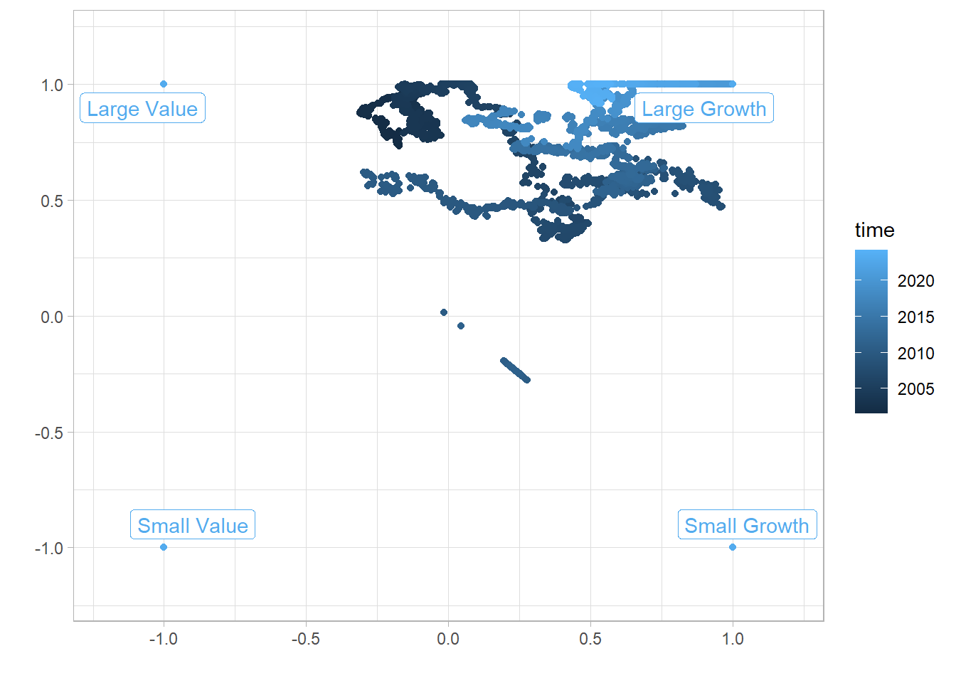
The plot highlights how the fund has changed over the years. In the beginning of our analysis period (2001) the fund was slightly leaning on the value side. Next it drifted down the size dimension and to the far edges of growth and then drifted over to growth, and then reversed course to a slight value tilt. More recently the style has skewed towards growth and the upper end of size. Reading the fund’s investment approach of measuring risk and relative performance vs. the S&P 500 this isn’t surprising. At the time of this writing mega cap growth stocks are significant driver of the S&P 500.
The rolling weights can be used to construct a tracking portfolio. We’ll shift the weights forward one day to assume a daily rebalance the day after our quadratic optimization. Take the results with a grain of salt, we’re not assuming any transaction fees or tax consequences of daily trading, the goal is to see if we can replicate the systematic sources of risk of the fund.
wgt_fwd <- na.omit(lag.xts(roll_xts, 1))
tracker_port <- rowSums(wgt_fwd * ret['2001-07-31/', 2:5])
cum_ret <- apply(cbind(tracker_port, ret['2001-07-31/', 1]) + 1, 2, cumprod)
wealth <- xts(cum_ret, zoo::index(ret['2001-07-31/']))
colnames(wealth) <- c('Tracker Port', 'FMAGX')
plot(wealth, legend.loc = 'topleft')
r2 <- cor(tracker_port, ret['2001-07-31/', 1])^2
paste0('r-squared ', round(r2 * 100, 1), '%')
[1] "r-squared 94.7%"Adaptability
Another nice feature about this framework is it can easily be adapted to other asset classes. For example fixed income funds can use duration, credit, and other relevant “styles”. This optimization can also be used with factor models to expand beyond value and size.